An Ordination Visualisation to Profile Training
Plot relationships between training drills based on athlete activity profile data using non-metric multidimensional scaling
Athlete activity profile data, such as that from global positioning systems (GPS) and accelerometers, is often used to quantify physical output during training1,2. This data may be aggregated to report the mean distances covered and speeds reached across training as a whole and within specific drills. Rather than simply reporting data this way, this edition of Visualising Athlete Data in R covers a technique that formed part of my Honours research (unpublished) to quantify and visualise the (dis)similarity between training drills based on physical output - as measured from GPS and accelerometers. Its hoped what’s covered here may add value to a practitioner’s decision making when designing training around specific activity targets (total distance, high-speed running etc.).
Non-metric multidimensional scaling
Its typical to profile training based on a variety of GPS- and accelerometer-derived variables, and we can use this multivariate data to spatially illustrate the relationships between different drills with non-metric multidimensional scaling (nMDS)3. Often used in ecology, nMDS is an ordination technique that takes a multivariate dataset and calculates the distances between samples and schematically represents the (dis)similarity in a two-dimensional space3. From an nMDS output we can get a sense of “likeness”, whereby similar training drills, for example, are located proximal to each other and dissimilar drills are observed further apart on an ordination plot3. This technique has previously been applied in sport to trace team match performance4, and it may also be useful in highlighting the (dis)similarity between drills that could aid the prescription of training. The following content will provide a (very) brief overview of how we can run nMDS in R using simulated GPS and accelerometer data. For a more comprehensive overview of nMDS, I encourage you to check out other resources online.
Example
Just as I have throughout my Visualising Athlete Data in R series, I’m simulating some data for the purpose of this example. The code below produces a 20 x 6 data frame containing drills and four commonly used variables describing the average physical output from each one. I’ve included the drill_type variable to colour the drill labels by their type when we eventually get to plotting.
library(tidyverse)

set.seed(450)
drill <- paste("Drill", 1:20)
drill_type <- rep(c("Passing & Receiving", "Running", "Defensive", "Tackling"),
                  each = 5)
tot_dist <- c(rnorm(20, 1000, 400))
metres_per_min <- c(rnorm(20, 100, 30))
hsr <- c(rnorm(20, 300, 100))
load_per_min <- c(rnorm(20, 12, 3))

dat <- data.frame(drill, drill_type, tot_dist, metres_per_min, hsr,
                  load_per_min)

dat <- dat %>% mutate_if(is.numeric, round)

head(dat)
## drill drill_type tot_dist metres_per_min hsr load_per_min
## 1 Drill 1 Passing & Receiving 1390 101 328 12
## 2 Drill 2 Passing & Receiving 933 86 147 14
## 3 Drill 3 Passing & Receiving 1025 84 265 12
## 4 Drill 4 Passing & Receiving 550 164 358 10
## 5 Drill 5 Passing & Receiving 1075 62 285 11
## 6 Drill 6 Running 1185 91 352 16Its important to keep in mind here that this dataset isn’t real and its use is only intended to illustrate the functionality of nMDS. If you’re collecting your own GPS and accelerometer data, you’ll most likely have this archived in a neatly formatted spreadsheet where the values will be much more representative of actual training than they are here.
In order to perform nMDS, our data frame needs to contain all numeric variables, so I’m dropping drill and drill_type momentarily using the - symbol in select() and will call on these again soon.
dat_num <- dat %>%
  select(-c(drill, drill_type))
Now we’re ready to run our nMDS analysis. To do this, I’m using the metaMDS() function from the vegan package, so make sure to install this if you haven’t already.
library(vegan)

set.seed(20)
nmds <- metaMDS(dat_num)
## Square root transformation
## Wisconsin double standardization
## Run 0 stress 0.1074252
## Run 1 stress 0.1074252
## ... Procrustes: rmse 0.0003488619 max resid 0.001203764
## ... Similar to previous best
## Run 2 stress 0.1074251
## ... New best solution
## ... Procrustes: rmse 0.0002179825 max resid 0.0007518953
## ... Similar to previous best
## Run 3 stress 0.1995752
## Run 4 stress 0.2134182
## Run 5 stress 0.163605
## Run 6 stress 0.1074251
## ... New best solution
## ... Procrustes: rmse 4.492981e-05 max resid 0.0001547674
## ... Similar to previous best
## Run 7 stress 0.1082238
## Run 8 stress 0.1890291
## Run 9 stress 0.1082239
## Run 10 stress 0.2393549
## Run 11 stress 0.1074251
## ... Procrustes: rmse 6.034984e-05 max resid 0.0002079273
## ... Similar to previous best
## Run 12 stress 0.1074251
## ... Procrustes: rmse 0.0001228853 max resid 0.000423898
## ... Similar to previous best
## Run 13 stress 0.1074251
## ... Procrustes: rmse 6.298803e-05 max resid 0.000215939
## ... Similar to previous best
## Run 14 stress 0.1074251
## ... Procrustes: rmse 0.0001134127 max resid 0.0003913605
## ... Similar to previous best
## Run 15 stress 0.1082238
## Run 16 stress 0.1082237
## Run 17 stress 0.2091802
## Run 18 stress 0.1074251
## ... Procrustes: rmse 0.0001119139 max resid 0.0003856809
## ... Similar to previous best
## Run 19 stress 0.163605
## Run 20 stress 0.1074251
## ... Procrustes: rmse 0.0001125207 max resid 0.0003853515
## ... Similar to previous best
## *** Solution reachedThe nMDS algorithm runs 20 times to find the smallest stress value which describes the goodness-of-fit of taking multidimensional data and squashing it down to only two dimensions. Lower stress values suggest a better fit of the data3, and here we have a stress of 0.107 representing a fair fit.
By calling str(), you’ll notice that nmds contains a list of a whole bunch of other objects.
str(nmds)## List of 35
## $ nobj : int 20
## $ nfix : int 0
## $ ndim : num 2
## $ ndis : int 190
## $ ngrp : int 1
## $ diss : num [1:190] 0.0154 0.0213 0.0227 0.0278 0.0286 ...
## $ iidx : int [1:190] 12 6 3 6 12 12 5 5 12 14 ...
## $ jidx : int [1:190] 6 3 1 5 7 5 3 1 3 1 ...
## $ xinit : num [1:40] 0.708 0.868 0.411 0.303 0.888 ...
## $ istart : int 1
## $ isform : int 1
## $ ities : int 1
## $ iregn : int 1
## $ iscal : int 1
## $ maxits : int 200
## $ sratmx : num 1
## $ strmin : num 1e-04
## $ sfgrmn : num 1e-07
## $ dist : num [1:190] 0.0307 0.0203 0.0452 0.0563 0.04 ...
## $ dhat : num [1:190] 0.0255 0.0255 0.0437 0.0437 0.0437 ...
## $ points : num [1:20, 1:2] -0.00833 0.09646 -0.00318 -0.06959 -0.03873 ...
## ..- attr(*, "dimnames")=List of 2
## .. ..$ : chr [1:20] "1" "2" "3" "4" ...
## .. ..$ : chr [1:2] "MDS1" "MDS2"
## ..- attr(*, "centre")= logi TRUE
## ..- attr(*, "pc")= logi TRUE
## ..- attr(*, "halfchange")= logi TRUE
## ..- attr(*, "internalscaling")= num 7.62
## $ stress : num 0.107
## $ grstress : num 0.107
## $ iters : int 145
## $ icause : int 3
## $ call : language metaMDS(comm = dat_num)
## $ model : chr "global"
## $ distmethod: chr "bray"
## $ distcall : chr "vegdist(x = comm, method = distance)"
## $ data : chr "wisconsin(sqrt(dat_num))"
## $ distance : chr "bray"
## $ converged : logi TRUE
## $ tries : num 20
## $ engine : chr "monoMDS"
## $ species : num [1:4, 1:2] 0.034001 -0.000461 -0.157215 0.121388 -0.141023 ...
## ..- attr(*, "dimnames")=List of 2
## .. ..$ : chr [1:4] "tot_dist" "metres_per_min" "hsr" "load_per_min"
## .. ..$ : chr [1:2] "MDS1" "MDS2"
## ..- attr(*, "shrinkage")= Named num [1:2] 0.0112 0.0112
## .. ..- attr(*, "names")= chr [1:2] "MDS1" "MDS2"
## ..- attr(*, "centre")= Named num [1:2] 2.33e-18 8.67e-19
## .. ..- attr(*, "names")= chr [1:2] "MDS1" "MDS2"
## - attr(*, "class")= chr [1:2] "metaMDS" "monoMDS"For visualising our mock training data, I only need the $points object from nmds which contains the positions in both MDS1 and MDS2 axes for each of the drills. I’m storing these points in a new data frame and rejoining the variables drill and drill_type from the original data.
plot_dat <- as.data.frame(nmds$points)

plot_dat$drill <- dat$drill
plot_dat$drill_type <- dat$drill_type

head(plot_dat)
## MDS1 MDS2 drill drill_type
## 1 -0.008325439 -0.058195970 Drill 1 Passing & Receiving
## 2 0.096458690 0.008543030 Drill 2 Passing & Receiving
## 3 -0.003175063 -0.013318578 Drill 3 Passing & Receiving
## 4 -0.069592025 0.123089054 Drill 4 Passing & Receiving
## 5 -0.038730410 -0.052840500 Drill 5 Passing & Receiving
## 6 -0.018653684 -0.000207782 Drill 6 RunningWe can now go ahead and start plotting!
Plot
Creating the nMDS plot is relatively straightforward once your data is set out correctly. Here’s the code.
library(RColorBrewer)
library(scales)

ggplot(data = plot_dat, aes(x = MDS1, y = MDS2, label = drill)) +
  geom_path(size = 0.1) +
  geom_label(aes(fill = drill_type), alpha = 0.6, color = "black",
             fontface = "bold") +
  scale_fill_manual(values = brewer.pal(name = "Set1", n = 4)) +
  scale_x_continuous(limits = c(-0.35, 0.15),
                     breaks = pretty_breaks(n = 8),
                     labels = number_format(accuracy = 0.01)) +
  scale_y_continuous(breaks = pretty_breaks(n = 5),
                     labels = number_format(accuracy = 0.01)) +
  theme_minimal() +
  guides(fill = guide_legend(title = "Drill Type",
                             title.position = "top",
                             title.hjust = 0.5,
                             override.aes = aes(label = ""))) +
  theme(panel.grid.minor = element_blank(),
        plot.background = element_rect(fill = "white", colour = NA),
        legend.position = "top",
        legend.title = element_text(face = "bold", size = 10),
        legend.text = element_text(size = 8),
        legend.key = element_rect(colour = "black"))
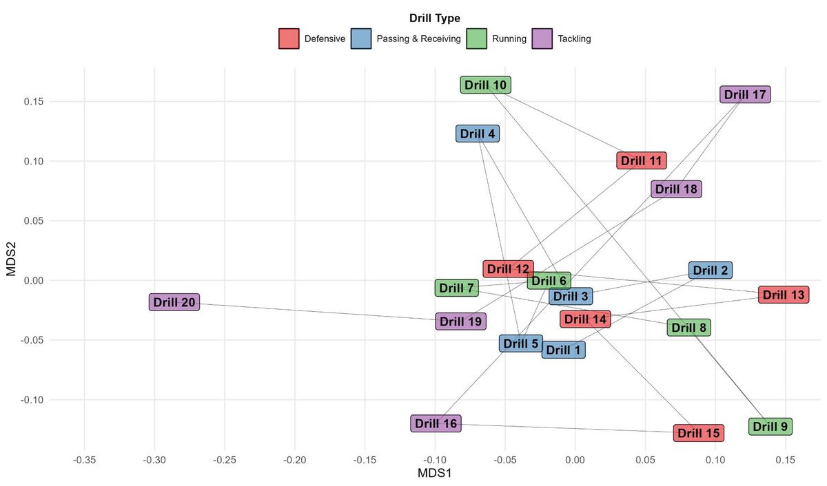
Here, I’m using geom_label() to plot the name of each drill in their respective position and, as alluded to above, applying a fill based on drill_type so we can see how these interact with each other also. I’m not personally a fan of the default colour scheme in ggplot2, so I’m using a different palette from the RColorBrewer package to customise this within scale_fill_manual(). The n = 4 in brewer.pal() represents the four different drill types so there’s a unique colour for each one. A neat function called number_format() from scales allows you to format the axis labels to the desired number of decimal places, where I’m using two (accuracy = 0.01) for consistency.
Interpretation
Drills that are clustered together on the ordination surface are similar based on the physical output they tend to elicit, whereas drills that are further apart, such as Drill 20 versus Drill 13, are dissimilar. In this mock example, we can say Drills 1, 3, 5, 6, 7, 12, 14 and 19 share an activity profile that is alike and we may expect the distances covered - including at high-speed - and accelerometer load accumulated to be similar amongst these drills. Conversely, despite Drills 16, 17, 18, 19 and 20 being tackling drills, they all produce a different physical output compared to one another based on their proximity on the plot.
Application
This is a relatively simple method to visualise the relationships between training drills using GPS and/or accelerometer data. A drill ordination plot may provide insight to coaches and practitioners about how athlete activity profile differs between drills and may be referred to when prescribing training.
If you collect GPS and/or accelerometer data during training and use this to profile your drills, give this plotting technique a try and hopefully it adds some value to your decision making around training prescription.
1. Boyd, L.J., K. Ball, and R.J. Aughey, Quantifying external load in Australian football matches and training using accelerometers. International Journal of Sports Physiology and Performance, 2013. 8(1): p. 44-51.
2. Corbett, D.M., et al., Development of physical and skill training drill prescription systems for elite Australian Rules football. Science and Medicine in Football, 2018. 2(1): p. 51-57.
3. Hout, M.C., M.H. Papesh, and S.D. Goldinger, Multidimensional scaling. Wiley Interdiscip Rev Cogn Sci, 2013. 4(1): p. 93-103.
4. Woods, C.T., et al., Non-metric multidimensional performance indicator scaling reveals seasonal and team dissimilarity within the National Rugby League. Journal of Science and Medicine in Sport, 2018. 21(4): p. 410-415.